Data cleaning and preprocessing are crucial steps in the data analysis process. They involve identifying and addressing issues and inconsistencies in the raw data to ensure its quality, accuracy, and suitability for further analysis. Proper data cleaning and preprocessing enhance the reliability and effectiveness of data analysis, machine learning models, and other data-driven tasks.

The data cleaning and preprocessing process typically include the following steps:

1. Handling Missing Data: Identify and handle missing values in the dataset. Missing data can be filled using imputation techniques, removing rows or columns with missing values, or using advanced imputation methods like k-nearest neighbors or regression imputation.
2. Handling Outliers: Outliers are data points that significantly deviate from the rest of the data. They can skew statistical analyses and machine learning models. Identify and deal with outliers appropriately, such as removing them, transforming them, or treating them as missing values.
3. Data Standardization/Normalization: If the data features have different scales, it is beneficial to standardize or normalize them to a common scale. Standardization scales the data to have a mean of 0 and a standard deviation of 1, while normalization scales the data to a specific range, such as [0, 1].
4. Encoding Categorical Data: Machine learning models typically require numeric inputs. Therefore, categorical variables need to be encoded into numerical representations using techniques like one-hot encoding, label encoding, or binary encoding.
5. Removing Redundant Features: Identify and remove features that do not contribute significantly to the analysis or introduce multicollinearity issues. Reducing the number of features can improve the model's efficiency and interpretability.
6. Feature Engineering: Create new features or transformations of existing features to provide more meaningful and informative representations of the data.
7. Handling Skewed Data: Address skewed distributions in the data using techniques like log transformation or box-cox transformation to improve the model's performance.
8. Data Integration: Combine multiple datasets or data sources, if needed, to create a more comprehensive dataset for analysis.
9. Data Type Conversion: Ensure that the data is in the correct data type for analysis and modeling.
10. Data Partitioning: Split the dataset into training, validation, and test sets for model training and evaluation.
11. Data Visualization: Visualize the data at different stages of cleaning and preprocessing to understand the effects of the transformations and to detect any further issues.

Data cleaning and preprocessing can be iterative processes, and different datasets may require specific techniques and approaches based on the nature of the data and the analysis goals. Properly cleaned and preprocessed data lays the foundation for accurate and meaningful data analysis and modeling, leading to more reliable insights and predictions.

Exploratory Data Analysis (EDA) is a critical step in the data analysis process that involves visually and quantitatively exploring the data to gain an initial understanding of its characteristics, patterns, and relationships. EDA helps data analysts and data scientists to identify potential issues, discover insights, and formulate hypotheses before applying more advanced statistical or machine learning techniques.

The primary goals of EDA are as follows:

1. Data Understanding: EDA aims to familiarize analysts with the structure, content, and context of the dataset. It involves examining the data's dimensions, data types, and basic statistics such as mean, median, standard deviation, minimum, maximum, etc.
2. Data Visualization: Visualizing the data through plots, charts, and graphs helps reveal patterns, trends, and anomalies that might not be apparent from raw data. Common visualization tools include scatter plots, bar charts, histograms, box plots, line charts, heatmaps, etc.
3. Data Quality Assessment: During EDA, analysts check for data quality issues, such as missing values, outliers, and inconsistencies. Addressing these issues is crucial before proceeding with any analysis.
4. Identifying Patterns and Relationships: EDA helps identify potential correlations, associations, or trends between different variables in the dataset. These insights can guide further analysis or inform the development of predictive models.
5. Feature Selection: For machine learning tasks, EDA can aid in selecting the most relevant features or variables that contribute significantly to the prediction or classification task.
6. Hypothesis Generation: By exploring the data, analysts can generate initial hypotheses about potential relationships between variables or identify interesting areas for further investigation.

Steps involved in Exploratory Data Analysis:

1. Data Collection: Gather the data from various sources, such as databases, files, or APIs.
2. Data Cleaning: Clean and preprocess the data to handle missing values, outliers, and inconsistencies.
3. Summary Statistics: Calculate basic statistics (mean, median, standard deviation, etc.) to gain a general understanding of the dataset.
4. Data Visualization: Create various plots and visualizations to explore patterns, distributions, and relationships in the data.
5. Correlation Analysis: Examine correlations between variables to identify potential dependencies.
6. Data Transformation: If necessary, perform transformations such as normalization or scaling to prepare the data for further analysis.
7. Insight Generation: Interpret the visualizations and summary statistics to generate insights and inform decision-making.

Exploratory Data Analysis is an iterative process, and the insights gained from EDA often influence the subsequent steps of data analysis, including model selection, feature engineering, and hypothesis testing. It is an essential step that lays the foundation for a more in-depth understanding of the data and ultimately aids in making informed decisions and drawing valuable insights from the dataset.

Data analysis problems can vary widely depending on the nature of the data, the objectives of the analysis, and the specific domain or industry. However, some common data analysis problems that arise in different fields include:

1. Exploratory Data Analysis (EDA): Understanding the structure, distribution, and basic characteristics of the data is often the first step in data analysis. EDA involves visualizing and summarizing data to identify patterns, trends, outliers, and potential relationships.
2. Data Cleaning and Preprocessing: Raw data may contain errors, missing values, duplicates, or inconsistencies that need to be addressed before conducting any analysis. Cleaning and preprocessing data are crucial to ensure data quality and accuracy.
3. Regression Analysis: Regression is used to model the relationship between one or more independent variables and a dependent variable. It is commonly used for predicting numerical outcomes and understanding the strength and direction of relationships.
4. Classification Problems: Classification involves categorizing data into predefined classes or categories. It is commonly used for tasks such as spam detection, sentiment analysis, image classification, and medical diagnosis.
5. Clustering: Clustering aims to group similar data points together based on their similarity. It is useful for data segmentation, customer segmentation, and pattern recognition.
6. Time-Series Analysis: Time-series data involves observations collected over time, and its analysis focuses on understanding temporal patterns, trends, and seasonality.
7. Anomaly Detection: Anomaly detection aims to identify rare events or data points that significantly deviate from the normal behavior of the dataset.
8. Text Analysis and Natural Language Processing (NLP): Analyzing text data involves tasks such as sentiment analysis, topic modeling, text classification, and named entity recognition.
9. Statistical Hypothesis Testing: Hypothesis testing is used to make inferences about a population based on a sample of data. It helps determine if observed differences between groups are statistically significant.
10. Data Visualization: Data visualization is crucial for presenting and communicating analysis results effectively. Choosing appropriate charts, graphs, and visual representations is essential for conveying insights clearly.
11. Dimensionality Reduction: Dimensionality reduction techniques like Principal Component Analysis (PCA) and t-distributed Stochastic Neighbor Embedding (t-SNE) help reduce the number of features while retaining the essential information.
12. Data Imputation: When dealing with missing data, imputation techniques are used to fill in the missing values based on patterns observed in the available data.

These are just a few examples of data analysis problems. The field of data analysis is vast, and the specific problems and techniques used will depend on the data, the questions being asked, and the objectives of the analysis. Data analysts and data scientists use a combination of statistical methods, machine learning algorithms, and domain expertise to tackle these challenges and derive valuable insights from data.

Softmax is an activation function used primarily in the output layer of multi-class classification neural networks. It takes a vector of raw, unnormalized scores and converts them into a probability distribution over the different classes. The output of the softmax function can be interpreted as the likelihood or probability of each class being the correct one.

The softmax function is defined as follows:

Given an input vector z = [z1, z2, ..., zn], the softmax function calculates the probability p_i for each element z_i as:

p_i = exp(z_i) / (exp(z1) + exp(z2) + ... + exp(zn))

Where:

exp is the exponential function, which raises the mathematical constant "e" (approximately 2.71828) to the power of the argument.

z_i represents the raw score or logit for the i-th class.

Key characteristics of the softmax function:

1. Probability distribution: The sum of all probabilities p_i will be equal to 1, ensuring that the output forms a valid probability distribution over the classes.
2. Amplifies differences: Softmax amplifies the differences between the scores, converting them into probabilities that emphasize the differences between classes. Higher scores will have correspondingly higher probabilities.
3. Output interpretation: The class with the highest probability is typically chosen as the predicted class by the model.

The softmax activation is particularly useful in multi-class classification tasks, where the neural network needs to predict a single class out of multiple possible classes. It is commonly used in conjunction with the cross-entropy loss function to train the neural network in such scenarios.

However, it is worth noting that softmax is not typically used in the hidden layers of the neural network, as it can make the model more susceptible to vanishing and exploding gradients during training. In the hidden layers, ReLU and its variants are commonly used for their ability to mitigate such issues.

In summary, softmax is a crucial activation function in multi-class classification neural networks, as it converts raw scores into meaningful class probabilities, allowing the model to make accurate predictions among multiple classes.

Python Implementation

To implement the softmax function in the python programming language, all you have to do is write the following code.

The result of running this code is shown in the original image at the top of the article. You can run the code in the following colab notebook: softmax activation function

Hyperbolic Tangent, commonly referred to as tanh, is an activation function frequently used in artificial neural networks. It is an extension of the sigmoid function but maps the input to a range between -1 and 1, making it zero-centered and capable of handling both positive and negative inputs. The tanh function exhibits stronger gradients around the origin compared to the sigmoid function, which can be advantageous during training.

The mathematical definition of the tanh activation function is as follows:

f(x) = (2 / (1 + exp(-2x))) - 1

Where:

x is the input to the function, which can be a single value or a vector (in the case of neural networks, it is usually the weighted sum of inputs to a neuron).

exp denotes the exponential function, which raises the mathematical constant "e" (approximately 2.71828) to the power of the argument.

Key characteristics of the tanh function:

1. Range: The output of tanh ranges from -1 to 1. When 'x' is large and positive, the function approaches 1, and when 'x' is large and negative, the function approaches -1. When 'x' is close to zero, the tanh function approaches zero.
2. Zero-centered: Unlike the sigmoid function, which has its midpoint at 0.5, tanh is zero-centered, meaning that its midpoint is at 0. This can be beneficial for optimization algorithms and helps avoid issues like vanishing gradients.

Advantages of tanh activation function:

1. Stronger gradients: The tanh function has steeper gradients around zero compared to the sigmoid function. This can facilitate faster learning and convergence during training.
2. Zero-centered output: Having a zero-centered output can help neural networks converge faster, especially in situations where the data distribution is centered around zero.

Despite its advantages, tanh shares some drawbacks with the sigmoid function, such as the potential for vanishing gradients for very large or very small inputs. In many cases, ReLU and its variants are preferred over tanh as activation functions in deep learning architectures due to their simplicity and better performance in avoiding vanishing gradients.

However, tanh can still be useful in specific cases, especially when a zero-centered output is desired or for certain network architectures where it performs well. As with all activation functions, the choice of tanh or other alternatives depends on the specific problem, the network's structure, and empirical experimentation to find the most suitable activation function for the given task.

Python Implementation

To implement the tanh function in the python programming language, all you have to do is write the following code.

The result of running this code is shown in the original image at the top of the article. You can run the code in the following colab notebook: tanh activation function

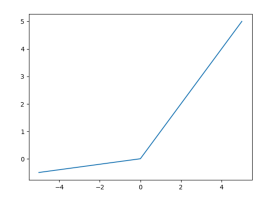
Leaky Rectified Linear Unit (Leaky ReLU) is a variant of the ReLU activation function that addresses the "dying ReLU" problem. The "dying ReLU" problem occurs when ReLU neurons become inactive for certain inputs during training, resulting in those neurons always outputting zero and not learning anything further.

Leaky ReLU introduces a small, non-zero slope for negative inputs, allowing the neurons to remain active even when the input is negative. The mathematical definition of Leaky ReLU is as follows:

f(x) = max(a*x, x)

Where:

x is the input to the function, which can be a single value or a vector (in the case of neural networks, it is usually the weighted sum of inputs to a neuron).

max takes the maximum value between a*x and x.

a is a small positive constant, usually a small fraction (e.g., 0.01).

When x is positive, Leaky ReLU behaves like the standard ReLU (f(x) = x). However, when 'x' is negative, it introduces a small negative slope determined by the value of a*x, which ensures that the neuron remains active and continues to learn, even for negative inputs.

The benefits of Leaky ReLU include:

1. Avoiding the "dying ReLU" problem: The small, non-zero slope for negative inputs prevents neurons from becoming inactive during training, promoting better learning and preventing the saturation of neurons.
2. Simplicity and computational efficiency: Like the standard ReLU, Leaky ReLU is computationally efficient and easy to implement.

In practice, Leaky ReLU is commonly used as an alternative to the standard ReLU activation function, especially when training very deep neural networks or models where the "dying ReLU" problem is likely to occur. However, the choice of activation function depends on the specific problem and architecture, and experimentation is often necessary to determine which activation function works best for a particular task. Other variants of ReLU, such as Parametric ReLU (PReLU), also allow the slope for negative inputs to be learned during training, offering more flexibility in the model's architecture.

Python Implementation

To implement the Leaky ReLU function in the python programming language, all you have to do is write the following code.

The result of running this code is shown in the original image at the top of the article. You can run the code in the following colab notebook: Leaky ReLU activation function

Rectified Linear Unit (ReLU) is a popular activation function used in artificial neural networks, especially in deep learning architectures. It addresses some of the limitations of older activation functions like the sigmoid and tanh functions. ReLU introduces non-linearity to the network and allows it to efficiently learn complex patterns and relationships within the data.

The ReLU activation function is defined as follows:

f(x) = max(0, x)

Where:

x is the input to the function, which can be a single value or a vector (in the case of neural networks, it is usually the weighted sum of inputs to a neuron).

max takes the maximum value between 0 and the input x.

The key characteristic of ReLU is that it is linear for positive inputs (f(x) = x) and zero for negative inputs (f(x) = 0). This simplicity makes it computationally efficient and easy to implement.

Advantages of ReLU:

1. Non-linearity: Although ReLU is linear for positive values, its output becomes non-linear for negative inputs, which introduces the necessary non-linearity to the neural network, enabling it to model complex relationships in the data.
2. Avoiding Vanishing Gradient: Unlike sigmoid and tanh functions, ReLU does not suffer from the vanishing gradient problem for positive inputs. This property helps in mitigating the training issues associated with very deep neural networks, as gradients do not diminish quickly during backpropagation.
3. Faster Convergence: ReLU activation leads to faster training of neural networks due to its simplicity and non-saturating behavior for positive values. This means that the neurons do not get stuck in regions with very small gradients during training.

Despite its advantages, ReLU has a limitation known as the "dying ReLU" problem. In this scenario, some neurons may become inactive during training and never activate again (outputting zero) for any input, which can hinder the learning process. To address this issue, variants of ReLU have been proposed, such as Leaky ReLU and Parametric ReLU, which allow small, non-zero gradients for negative inputs, ensuring that neurons remain active during training.

In summary, ReLU is a widely used activation function that has significantly contributed to the success of deep learning models, especially in computer vision tasks. It is computationally efficient, helps in mitigating vanishing gradient problems, and accelerates the training process. However, practitioners should be aware of the "dying ReLU" problem and consider using its variants when appropriate.

Python Implementation

To implement the ReLU function in the python programming language, all you have to do is write the following code.